Advanced Analytics for a Big Data World

# Advanced Analytics for a Big Data World (2026) This page contains slides, references and materials for the "Advanced Analytics for a Big Data World" course. *Last updated at 2026-05-04* # Table of contents

# Course 1: February 9 ## Slides * [About the Course](./slides/00-About.pdf) * [Introduction](./slides/01-Introduction.pdf) ## Assignment Information The evaluation of this course consists of a lab report (50% of the marks) and a closed-book written exam with both multiple-choice and open questions (50% of the marks). * Your lab-report will consist of your write-ups of four assignments, which will be made available throughout the semester * You will work in groups of five students * The four assignments consist of (1) Predictive model competition using R or Python (tabular); (2) Deep learning application (imagery); (3) Text mining with generative AI (text); (4) Social network/graph analytics assignment (network) * Per assignment, you describe your results (screen shots, numbers, approach); more detailed information will be provided per assignment * You do not hand in each assignment separately, but hand in your completed lab report containing all four assignments on Sunday May 31st **For forming groups, please see the Toledo page after the first course.** **Note for externals (i.e. anyone who will NOT partake in the exams -- this doesn't apply to normal students)**: you are free to partake in (any of) the assignments individually (they'll be posted on this page as well), but not required to. ## Recording * [YouTube](https://youtu.be/YObDLUDqORo) ## Background Information Extra references: * [Deepmind blog](https://deepmind.google/blog/) * [OpenAI blog](https://openai.com/index/) * [Anthropic research blog](https://www.anthropic.com/research/) * [Qwen Coder Next](https://qwen.ai/blog?id=qwen3-coder-next) * [Kimi K2](https://moonshotai.github.io/Kimi-K2/thinking.html) * [Your brain on ChatGPT](https://www.media.mit.edu/publications/your-brain-on-chatgpt/) * [AlphaGo](https://www.engadget.com/2016-03-14-the-final-lee-sedol-vs-alphago-match-is-about-to-start.html) and their newer ["AlphaGo Zero"](https://deepmind.com/blog/alphazero-shedding-new-light-grand-games-chess-shogi-and-go/) * [AlphaStar](https://deepmind.com/blog/alphastar-mastering-real-time-strategy-game-starcraft-ii/) * [AlphaFold](https://deepmind.com/blog/article/AlphaFold-Using-AI-for-scientific-discovery) and a [recent article where it was used](https://arxiv.org/abs/2201.09647) * [AlphaCode](https://alphacode.deepmind.com/) * [DALL·E: Creating Images from Text](https://openai.com/blog/dall-e/) * [Automating My Job with GPT-3](https://blog.seekwell.io/gpt3) * [Stable Diffusion](https://stability.ai/blog/stable-diffusion-public-release) * [ChatGPT](https://openai.com/blog/chatgpt/) * [Millions of new materials discovered with deep learning](https://deepmind.google/discover/blog/millions-of-new-materials-discovered-with-deep-learning/) * [AlphaGeometry](https://deepmind.google/discover/blog/alphageometry-an-olympiad-level-ai-system-for-geometry/) * [DeepSeek expained](https://heidloff.net/article/deepseek-r1/) and [announcement](https://github.com/deepseek-ai/DeepSeek-R1) * [Janus Pro is DeepSeek's image generator](https://huggingface.co/deepseek-ai/Janus-Pro-7B) * [Kimi](https://github.com/MoonshotAI/Kimi-k1.5) and [Qwen](https://github.com/QwenLM/Qwen) * [Hunyuan3D-2](https://github.com/Tencent/Hunyuan3D-2) * [The Economics of AI Today](https://thegradient.pub/the-economics-of-ai-today/) * [Designing great data products: The Drivetrain Approach: A four-step process for building data products](https://www.oreilly.com/radar/drivetrain-approach-data-products/) * [Google's Rules of ML](https://developers.google.com/machine-learning/guides/rules-of-ml) * [150 successful machine learning models: 6 lessons learned at Booking.com](https://blog.acolyer.org/2019/10/07/150-successful-machine-learning-models/) -- recommended read! * The tank story: [how much is true?](https://www.gwern.net/Tanks) * [Self-driven car spins in circles](https://twitter.com/mat_kelcey/status/886101319559335936) * [Correlation is not causation](https://web.archive.org/web/20210413060837/http://robertmatthews.org/wp-content/uploads/2016/03/RM-storks-paper.pdf) * [Once billed as a revolution in medicine, IBM’s Watson Health is sold off in parts](https://www.statnews.com/2022/01/21/ibm-watson-health-sale-equity/) * [How To Break Anonymity of the Netflix Prize Dataset](https://arxiv.org/abs/cs/0610105) * [Why UPS drivers don’t turn left and you probably shouldn’t either](http://www.independent.co.uk/news/science/why-ups-drivers-don-t-turn-left-and-you-probably-shouldn-t-either-a7541241.html) # Course 2: February 16 ## Slides * [Supervised Essentials I](./slides/02-Supervised-1.pdf) ## Recording * [YouTube](https://youtu.be/BFi-FQGL4s8) ## Background Information [In the news](./news/News_02-16.pptx) (slides) Extra references on preprocessing: * [Forecasting with Google Trends](https://medium.com/dataminingapps-articles/forecasting-with-google-trends-114ab741bda4) * [Google Street View in insurance](https://arxiv.org/ftp/arxiv/papers/1904/1904.05270.pdf) * [Predicting the State of a House Using Google Street View](https://link.springer.com/chapter/10.1007/978-3-031-05760-1_46) * Packages for missing value summarization: [missingno](https://github.com/ResidentMario/missingno) and [VIM](https://cran.r-project.org/web/packages/VIM/index.html) * [MICE is also a popular package for dealing with missing values in R](https://www.r-bloggers.com/imputing-missing-data-with-r-mice-package/) * [More on data "leakage" and why you should avoid it](https://www.kaggle.com/alexisbcook/data-leakage) * [Another excellent presentation on the types of data leakage](https://www.slideshare.net/YuriyGuts/target-leakage-in-machine-learning) * [`smbinning`, an R package for weights of evidence encoding](https://cran.r-project.org/web/packages/smbinning/index.html) * [`category_encoders`: an interesting package containing a wide variety of categorical encoding techniques](http://contrib.scikit-learn.org/category_encoders/) * [More on the leave one out mean](https://www.kaggle.com/c/caterpillar-tube-pricing/discussion/15748) as discussed on Kaggle * [More explanation on the hashing trick on Wikipedia](https://en.wikipedia.org/wiki/Feature_hashing) * [Feature Hashing in Python](https://scikit-learn.org/stable/modules/generated/sklearn.feature_extraction.FeatureHasher.html) * [Entity Embeddings of Categorical Variables](https://arxiv.org/pdf/1604.06737.pdf) * [`dm` R package](https://krlmlr.github.io/dm/) * [`skrub`: Prepping tables for machine learning](https://github.com/skrub-data/skrub) * [`featuretools`: An open source python framework for automated feature engineering](https://www.featuretools.com/) * See also [`stumpy`](https://github.com/TDAmeritrade/stumpy) and [`tsfresh`](https://tsfresh.readthedocs.io/) * [AutoFeat](https://github.com/cod3licious/autofeat) * [FeatureSelector](https://github.com/WillKoehrsen/feature-selector) * [OneBM](https://arxiv.org/abs/1706.00327) * [More information on principal component analysis (PCA)](http://setosa.io/ev/principal-component-analysis/) * [OpenCV](http://opencv.org/) (for feature extraction from facial images), or see [this page](https://github.com/ageitgey/face_recognition) * Interesting application of PCA to "understand" the latent features of a deep learning network: [https://www.youtube.com/watch?v=4VAkrUNLKSo](https://www.youtube.com/watch?v=4VAkrUNLKSo) * [Another application of PCA for understanding model outputs](https://github.com/asabuncuoglu13/sketch-embeddings) Extra references on supervised basics: * [“Building Bridges between Regression, Clustering, and Classification”](https://arxiv.org/abs/2502.02996) * [Frank Harell on stepwise regression](https://www.stata.com/support/faqs/statistics/stepwise-regression-problems/) * [Stepwise feature selection in scikit-learn](https://scikit-learn.org/stable/modules/feature_selection.html#sequential-feature-selection) but note that it applies cross validation * [L1 and L2 animation](https://nitter.net/itayevron/status/1328421322821693441) * [aerosolve - Machine learning for humans](https://medium.com/airbnb-engineering/aerosolve-machine-learning-for-humans-55efcf602665) * [ID3.pdf](./papers/ID3.pdf) and [C45.pdf](./papers/C45.pdf): extra material regarding decision trees * [Nice video on Entropy and Information](https://www.youtube.com/watch?v=v68zYyaEmEA) * [CloudForest](https://github.com/ryanbressler/CloudForest), an older but interesting decision tree ensemble implementation with support for three-way splits to deal with missing values, implemented in... Go * [RIPPER](https://christophm.github.io/interpretable-ml-book/rules.html), [RuleFit](https://github.com/christophM/rulefit) and [Skope-Rules](https://github.com/scikit-learn-contrib/skope-rules) * [dtreeviz](https://github.com/parrt/dtreeviz) for nicer visualizations or [pybaobabdt](https://pypi.org/project/pybaobabdt/) * White box models can be easily deployed, even in Excel... For some fun examples, see [m2cgen](https://github.com/BayesWitnesses/m2cgen), which can convert ML models to Java, C, Python, Go, PHP, ..., [emlearn](https://github.com/emlearn/emlearn) converts ML code to portable C99 code for microcontrollers, [sklearn-porter](https://github.com/nok/sklearn-porter) converts scikit-learn models to C, Java and others, and [SKompiler](https://github.com/konstantint/SKompiler) converts scikit-learn models to SQL queries, and... Excel * Two newer examples using k-NN: [1](https://towardsdatascience.com/scanned-digits-recognition-using-k-nearest-neighbor-k-nn-d1a1528f0dea) and [2](https://medium.com/learning-machine-learning/recommending-animes-using-nearest-neighbors-61320a1a5934) # Course 3: February 23 ## Slides * [Supervised Essentials II](./slides/03-Supervised-2.pdf) ## Recording * [YouTube](https://youtu.be/8uZy_75YHv4) ## Background Information [In the news](./news/News_02-23.pptx) (slides) Extra references: * [ROSE](https://cran.r-project.org/web/packages/ROSE/index.html) is a popular package for dealing with over/undersampling in R * [imblearn](https://imbalanced-learn.org/stable/) contains many smart sampling implementations for Python * [Tuning Imbalanced Learning Sampling Approaches](https://www.dataminingapps.com/2019/06/tuning-imbalanced-learning-sampling-approaches/) * More on the ROC curve: [1](https://arxiv.org/pdf/1812.01388.pdf), [2](http://www.rduin.nl/presentations/ROC%20Tutorial%20Peter%20Flach/ROCtutorialPartI.pdf), [3](https://stats.stackexchange.com/questions/225210/accuracy-vs-area-under-the-roc-curve/225221#225221) * [Averaging ROC curves for multiclass](https://scikit-learn.org/stable/auto_examples/model_selection/plot_roc.html) * [The Relationship Between Precision-Recall and ROC Curves](./papers/rocpr.pdf): a paper by KU Leuven's Jesse Davis et al. on the topic with some other interesting remarks * [h-index.pdf](./papers/h-index.pdf): paper regarding the h-index as an alternative for AUC * [BSZ tuning](./papers/bsztuning.pdf): paper on BSZ tuning: a simple cost-sensitive regression approach * [A blog post explaining cross validation](https://towardsdatascience.com/train-test-split-and-cross-validation-in-python-80b61beca4b6) * [Multiclass and multilabel algorithms in scikit-learn](https://scikit-learn.org/stable/modules/multiclass.html) * [scikit.ml](http://scikit.ml/) contains more advanced multilabel techniques * More on probability calibration [here](http://scikit-learn.org/stable/modules/calibration.html) and [here](http://fastml.com/classifier-calibration-with-platts-scaling-and-isotonic-regression) * [More on the System Stability Index](https://www.dataminingapps.com/2016/10/what-is-a-system-stability-index-ssi-and-how-can-it-be-used-to-monitor-population-stability/) * [Visibility and Monitoring for Machine Learning Models](http://blog.launchdarkly.com/visibility-and-monitoring-for-machine-learning-models/) * [What's your ML test score? A rubric for production ML systems](https://research.google.com/pubs/pub45742.html) * [Hidden Technical Debt in Machine Learning Systems](https://papers.nips.cc/paper/5656-hidden-technical-debt-in-machine-learning-systems) ## Assignment 1 In this assignment, you will construct a predictive model to predict the future revenue of customers of a European fashion shop. The data set is centered around online (web shop) sales of shoes. The data set can be downloaded through Toledo. Student groups will play "competitively" using [this website](https://seppe.net/aa/assignment1/) * **You will have received a password and your final group number through an email, which you need to make submissions**; in case of issues, contact me as soon as possible * The test set does not contain the target, so you will need to split up the train set accordingly to create your own validation set. The test set supplied in the data is used to rank and assess your model on the competition leaderboard * Your model will be evaluated using two metrics: Mean Absolute Error and Spearman Correlation as a secondary score * Note that only about half of the test set is used for the "public" leaderboard. That means that the score you will see on the leaderboard is done using this part of the test only (you don't know which half). Later on through the semester, submissions are frozen and the resuls on the "hidden" part will be revealed * Outliers, noisy data, missing values, and the heavy featurization you will have to perform will make for challenges to be overcome * The results of your latest submission are used to rank you on the leaderboard. This means it is your job to keep track of different model versions / approaches / outputs in case you'd like to go back to an earlier result * Once the hidden leaderboard is revealed, you should reflect on both results and explain accordingly in your report. E.g. if you did well on the public leaderboard but not on the hidden one, what might have caused this? The idea is not that you then step in and "fix" your model, but to learn and reflect * Also, whilst you can definitely try, the goal is not to "win", but to help you reflect on your model's results, see how others are doing, etc. * Your model needs to be build using Python (or R, Go, Rust, Julia or whatever you prefer as long as it involves coding). As an environment, you can use e.g. Jupyter (Notebook or Lab), RStudio, Google Colaboratory, Microsoft Azure Machine Learning Studio... and any additional library or package you want * Feel free to use ChatGPT, but try to make sure you know what you are doing **Data** Note that the data set contains the following files: - `transactions.csv`: transactions (purchases) during the feature construction period (y1-y2). Note that the same customer can obviously have made multiple purchases. You will need to use this to construct informative features - `customer_clv_train.csv`: revenue for each train set customer during the target observation period (y3-y4) - `customer_clv_test.csv`: the test customers you need to predict the revenue for during the same target observation period The train/test split was made out of sample instead of out of time. This is not ideal but was the only option as not enough data was available to construct transactions and targets over a longer time span. The data set was already minimally pre-processed and anonymized where necessary, but probably a lot of processing remains. Tip: first perform a thorough exploration of the data set. You will note that there is a large group of customers that do not generate any revenue during the target observation period, meaning that they shopped in y1-y2, but did not come back. Think how you can incorporate this effectively in your modelling pipeline. The features for each transaction are as follows: - `cust_id`: unique identifier of the customer placing the order - `order_date`: date when the order was placed - `pack_date`: date when the order was packed/shipped - `sale_id`: unique identifier of the sales transaction (multiple articles can be present in the same transaction) - `sale_discount_applied`: monetary value of discount applied to the sale - `sale_revenue`: final revenue amount received for this line item after discount - `returned_to_shop_id`: identifier of the shop/location where the item was returned (empty if not returned) - `prod_id`: unique identifier of the purchased product - `prod_size`: shoe size of the product - `prod_web_only`: binary flag (1/0) indicating whether the product is sold online only - `prod_season`: season or collection code (e.g., W14 = Winter 2014) - `prod_brand`: brand name of the product - `prod_title`: full commercial product name/title - `prod_color`: primary color of the product - `prod_type_1`: primary target group or category (e.g., men, women, boys) - `prod_type_2`: not included (= "shoes") - `prod_type_3`: secondary product category (e.g., sneakers, high shoes) - `prod_type_4`: tertiary style classification (e.g., high-top sneakers) - `prod_type_5`: additional style descriptor (e.g., boots with velcro, dress boots) - `prod_heel`: heel type or heel specification (if known) - `prod_material`: main outer material of the shoe (e.g., leather, suede) (if known) - `prod_insole`: indicator of specific insole feature (if known) - `prod_print`: type of print or pattern (if known) - `prod_comfort_sole`: indicator of special comfort sole feature (if known) - `prod_comfort_wear`: indicator of enhanced comfort wear feature (if known) - `prod_clasp`: type of closing mechanism (e.g., velcro, zipper, lace-up) (if known) - `prod_outlet`: indicator how often this product was sold through an outlet channel, higher values indicate that the product appeared more often **Deliverables** * Feel free to include code fragments, tables, visualisations, etc. * Some groups prefer to write their final report using Jupyter Notebook, which is fine, as long as it is readable top-to-bottom * You can use any predictive technique/approach you want, though focus on the whole process: general setup, critical thinking, and the ability to get and validate an outcome * You're free to use unsupervised technique for your data exploration part, too. When you decide to build a black box model, including some interpretability techniques to explain it is a nice idea * Any other assumptions or insights are thoughts can be included as well: the idea is to take what we've seen in class, get your hands dirty and try out what we've seen **Important: All groups should submit the results of their predictive model at least once to the leaderboard before the hidden scores are revealed (I'll warn you in time)** More info on how to submit can be found on the [submission website](https://seppe.net/aa/assignment1/). *You do not hand in each assignment separately, but hand in your completed lab report containing all four assignments on Sunday May 31st. For an overview of the groups, see Toledo. Note for externals (i.e. anyone who will NOT partake in the exams -- this doesn't apply to normal students): you are free to partake in (any of) the assignments individually, but not required to.* # Course 4: March 2 ## Slides * Same as last week ## Recording * [YouTube](https://youtu.be/Xf-LtVoivNM) ## Background Information [In the news](./news/News_03-02.pptx) (slides) Extra references on interpretability: * [Fantastic book on the topic of interpretability](https://christophm.github.io/interpretable-ml-book/) * [http://explained.ai/rf-importance/index.html](Beware of using feature importance!) * [https://academic.oup.com/bioinformatics/article/26/10/1340/193348](Permutation importance: a corrected feature importance measure) * [Interpreting random forests: Decision path gathering](http://blog.datadive.net/interpreting-random-forests/) * [Local interpretable model-agnostic explanations](https://github.com/marcotcr/lime) * [SHAP (SHapley Additive exPlanations)](https://github.com/slundberg/shap) * [Another great overview](https://github.com/jphall663/awesome-machine-learninginterpretability) * [rfpimp package](https://pypi.org/project/rfpimp/) * [Forest floor](http://forestfloor.dk/) for higher-dimensional partial depence plots * [The pdp R package](https://cran.r-project.org/web/packages/pdp/pdp.pdf) * [The iml R Package](https://cran.r-project.org/web/packages/iml/index.html) * [Descriptive mAchine Learning EXplanations (DALEX) R Package](https://github.com/pbiecek/DALEX) * [eli5 for Python](https://eli5.readthedocs.io/en/latest/index.html) * [Skater for Python](https://github.com/datascienceinc/Skater) * scikit-learn has Gini-reduction based importance but permutation importance has [been added in recent versions](https://scikit-learn.org/stable/modules/permutation_importance.html) * Or with [https://github.com/parrt/random-forest-importances](https://github.com/parrt/random-forest-importances) * Or with [https://github.com/ralphhaygood/sklearn-gbmi](https://github.com/ralphhaygood/sklearn-gbmi) (sklearn-gbmi) * [pdpbox for Python](https://github.com/SauceCat/PDPbox) * [vip for Python (and R)](https://koalaverse.github.io/vip/index.html) * [https://medium.com/@Zelros/a-brief-history-of-machine-learning-models-explainability-f1c3301be9dc](https://medium.com/@Zelros/a-brief-history-of-machine-learning-models-explainability-f1c3301be9dc) * Graft, Reassemble, Answer delta, Neighbour sensitivity, Training delta (GRANT) - [https://github.com/wagtaillabs](https://github.com/wagtaillabs) * [Classification Acceleration via Merging Decision Trees](./papers/mergingtrees.pdf) # Course 5: March 9 ## Slides * [Supervised Essentials III](./slides/04-Supervised-3.pdf) * [Deep Learning I](./slides/05-DeepLearning-1.pdf) ## Recording * [YouTube](https://youtu.be/s5gitU4dQb8) ## Background Information [In the news](./news/News_03-09.pptx) (slides) Extra references on ensemble models: * The [jar of jelly beans](https://towardsdatascience.com/the-unexpected-lesson-within-a-jelly-bean-jar-1b6de9c40cca) * The [documentation of scikit-learn](http://scikit-learn.org/stable/modules/ensemble.html) is very complete in terms of ensemble modeling * Kaggle post on [model stacking](http://blog.kaggle.com/2016/12/27/a-kagglers-guide-to-model-stacking-in-practice/) * [Random forest.pdf](./papers/Random forest.pdf): the original paper on random forests * [ExtraTrees](https://scikit-learn.org/stable/modules/ensemble.html#forest): "In extremely randomized trees (see ExtraTreesClassifier and ExtraTreesRegressor classes), randomness goes one step further in the way splits are computed. As in random forests, a random subset of candidate features is used, but instead of looking for the most discriminative thresholds, thresholds are drawn at random for each candidate feature and the best of these randomly-generated thresholds is picked as the splitting rule" * Also interesting to note is that scikit-learn's implementation of decision trees (and random forest) supports [multi-output problems](https://scikit-learn.org/stable/modules/tree.html#tree-multioutput) * Note that some implementations/papers for ExtraTrees will go a step further and simply select a splitting point completely at random (e.g. the subset of thresholds is size 1 -- this is helpful when working with very noisy features) * [To tune or not to tune the number of trees in a random forest](./papers/tune_or_not.pdf); conclusions: use a sufficiently high amount of trees * [Adaboost.pdf](./papers/Adaboost.pdf): the original paper on AdaBoost * [alr.pdf](./papers/alr.pdf): Friedman's paper on AdaBoost and Additive Logistic Regression * [xgboost documentation](https://xgboost.readthedocs.io/en/latest/) with a good [introduction](https://xgboost.readthedocs.io/en/latest/tutorials/model.html) * [lightgbm documentation](https://lightgbm.readthedocs.io/en/latest/pythonapi/) * [catboost documentation](https://catboost.ai/en/docs/) * Note that all three of these have sklearn-API compatible classifiers and regressors, so you can combine them with other typical sklearn steps # Course 6: March 16 ## Slides * Continuing with the slides of last time ## Recording * [YouTube](https://youtu.be/WZZSWOHXaO0) ## Background Information [In the news](./news/News_03-16.pptx) (slides) Extra references: * [Keras Vision tutorials - use these to get started with assignment 2!](https://keras.io/examples/vision/) * [A brief history of AI](https://beamandrew.github.io/deeplearning/2017/02/23/deep_learning_101_part1.html) * [Who invented the reverse mode of differentiation](https://www.math.uni-bielefeld.de/documenta/vol-ismp/52_griewank-andreas-b.pdf) * [Backpropagation explained](http://home.agh.edu.pl/~vlsi/AI/backp_t_en/backprop.html) * [Great short YouTube playlist explaining ANNs (3blue1brown)](https://www.youtube.com/watch?v=aircAruvnKk&list=PLZHQObOWTQDNU6R1_67000Dx_ZCJB-3pi) * [And other one explaining convolutions (3blue1brown)](https://www.youtube.com/watch?v=8rrHTtUzyZA ) * [Introduction to neural networks](https://victorzhou.com/blog/intro-to-neural-networks/) * [Tensorflow playground](https://playground.tensorflow.org/) * [NeuroEvolution of Augmenting Topologies (NEAT)](https://en.wikipedia.org/wiki/Neuroevolution_of_augmenting_topologies) * In class, I mentioned some recent papers around the bias-variance double descent phenomenon. [Chatterjee, S., & Zielinski, P. (2022). On the generalization mystery in deep learning](https://arxiv.org/abs/2203.10036) and especially [Wilson, A. G. (2025). Deep Learning is Not So Mysterious or Different](https://arxiv.org/abs/2503.02113) are interesting to read ## Assignment 2 In this assignment, you will construct a deep learning model to predict a target on a data set of Lego Minifigs (mini figures). The data was obtained from [brickset.com](https://brickset.com). **Data** * The set of images can be downloaded [using this link](https://e.pcloud.link/publink/show?code=XZYQmGZwIUEyLDBKRmnOsRuq4zub5BpRs2X) * You will also need [this json file](./assignment2/minifigs.json) containing the metadata The JSON file has an entry for each image looking e.g. like this: ``` { "id": 2, "name": "LEGOLAND - Black Torso, Black Legs, Black Hat", "link": "/minifigs/old011/legoland-black-torso-black-legs-black-hat", "year": 1975, "img_url": "https://img.bricklink.com/ItemImage/MN/0/old011.png", "minifig_number": "OLD011", "category": "LEGOLAND", "subcategory": "General", "year_released": "1975", "set_id": "7 sets", "current_value_new": "Not known", "current_value_used": "~\u20ac1.53", "character_name": null, "img_local_path": "images/OLD011.jpg", "themes": ["Basic", "LEGOLAND", "Universal Building Set"] }, ``` Note: the `\u20ac` stands for the EUR currency sign. **Objective** Your task is to construct a deep learning model to predict one of the following (you can choose what you find most interesting to work on): * Multiclass: try to predict the category based on the image * Multilabel: try to predict which "themes" are present (a bit harder) * Regression: try to predict the year of release, or the "value" of the mini figure (this is probably harder to do but can also be fun) If you find the classes or labels too large, you can also decide to focus on the top-k most occurring ones instead. Split the data set into train / val / test sets in a careful manner. Pick an evaluation metric to report on in accordance with the chosen task. **Tips** * You can train a model from scratch, but fine-tuning an existing image is probably a good idea * Try using an interpretability technique to figure out what your model is focusing on * Check the tutorials on [https://keras.io/examples/vision/](https://keras.io/examples/vision/) * You can use any deep learning library you want, but Keras or PyTorch will probably be easiest **Deliverables** * Overview of your full pipe line, including architecture, trade-offs, ways used to prevent overfitting, etc. * Results based on your chosen evaluation metric * Illustration of your model's predictions on a couple of test images *You do not hand in each assignment separately, but hand in your completed lab report containing all four assignments on Sunday May 31st. For an overview of the groups, see Toledo. Note for externals (i.e. anyone who will NOT partake in the exams -- this doesn't apply to normal students): you are free to partake in (any of) the assignments individually, but not required to.* # Course 7: March 23 ## Slides * Continuing with the slides of last time ## Recording * [YouTube](https://youtu.be/6kjVUeeJs5k) ## Background Information [In the news](./news/News_03-23.pptx) (slides) # Course 8: March 30 ## Slides * [Unsupervised Learning](./slides/06-Unsupervised.pdf) ## Recording * [YouTube](https://youtu.be/roLJn0QUuRE) ## Background Information [In the news](./news/News_03-30.pptx) (slides) Extra references: * [Comparing different hierarchical linkage methods on toy datasets](https://scikit-learn.org/stable/auto_examples/cluster/plot_linkage_comparison.html#sphx-glr-auto-examples-cluster-plot-linkage-comparison-py) * [Visualisation of the DBSCAN clustering technique in the browser](https://www.naftaliharris.com/blog/visualizing-dbscan-clustering/) * [More on the Gower distance](https://medium.com/@rumman1988/clustering-categorical-and-numerical-datatype-using-gower-distance-ab89b3aa90d9) * [Self-Organising Maps for Customer Segmentation using R](https://www.r-bloggers.com/self-organising-maps-for-customer-segmentation-using-r/) * [t-SNE](https://lvdmaaten.github.io/tsne/) and using it for [anomaly detection](https://medium.com/@Zelros/anomaly-detection-with-t-sne-211857b1cd00) * [http://distill.pub/2016/misread-tsne/](http://distill.pub/2016/misread-tsne/) provides very interesting visualisations and more explanation on t-SNE * [Be careful when clustering the output of t-SNE](https://stats.stackexchange.com/questions/263539/clustering-on-the-output-of-t-sne/264647#264647) * [UMAP](https://umap-learn.readthedocs.io/en/latest/how_umap_works.html) * [PixPlot](https://dhlab.yale.edu/projects/pixplot/): another cool example of t-SNE (this was the name I was trying to recall during class) * [Isolation forests](https://scikit-learn.org/stable/auto_examples/plot_anomaly_comparison.html#sphx-glr-auto-examples-plot-anomaly-comparison-py) * [Local outlier factor](https://scikit-learn.org/stable/auto_examples/neighbors/plot_lof_outlier_detection.html#sphx-glr-auto-examples-neighbors-plot-lof-outlier-detection-py) * [Twitter's anomaly detection package](https://github.com/twitter/AnomalyDetection) and [prophet](https://facebook.github.io/) * [An interesting article on detecting NBA all-stars using CADE](http://darrkj.github.io/blog/2014/may102014/) * Papers on [DBSCAN](./papers/dbscan.pdf), [isolation forests](./papers/iforest.pdf) and [CADE](./papers/CADE.pdf) # Course 9: April 20 ## Slides * [Deep Learning II](./slides/07-DeepLearning-2.pdf) ## Recording * [YouTube](https://youtu.be/moTpcPYq8iE) ## Assignment 3 In this assignment, you will construct a recommender system for games on Steam using LLMs. **Data** The starter code and data set can be downloaded [here](https://e.pcloud.link/publink/show?code=XZJJKvZhFNlwL1CXnzFnsC6JVGVwXSLn3tV). The zip file contains a `README.MD` file with more information. Extract the zip file to a folder of your choice. Data about games on the Steam store was scraped up until the beginning of April 2026. Only games with more than 25 reviews were kept in the data set. For each game, only the most recent 500 English reviews where scraped. The data was saved in a sqlite database (`steam_games_reviews_25.sqlite`) in these tables: - `games`: game data - `reviews`: user reviews The starter code consists of a simple Flask web app (a single frontend page and some backend API endpoints) and a dummy implementation of a recommender system. **Objective** The file `recommender.py` contains a dummy scaffold implementation. Your task is to extend this scaffold and create an LLM-driven recommender engine. - You will most likely need an embedding model to embed the game information in vectors - You might want to store these in a vector database for faster lookup - Then craft a prompt to give to an LLM with the retrieved context - You can also incorporate the `reviews` table if you want recommendations grounded in player feedback instead of game data alone - You can add whatever Python package you want to this repo (`uv add `) You don't need to use a cloud LLM provider, you can call models running in a local [Ollama](https://ollama.com/download) installation, and small models such as Phi 3.5 or the recent Gemma 4 will probably work well enough for this task. Open `recommender.py`, read the comments and replace: - `retrieve_candidates()` - `rank_candidates()` - `generate_answer()` Keep the JSON shape returned by `search()` the same so the Flask API and frontend continue to work. Feel free to make other modifications, but make sure the Flask app can be properly started. Both the web frontend and the API backend will be used to check your recommendations. If your note very familiar with games and want to check if your recommendations make sense, you can check out the [Steam Store](https://store.steampowered.com/), which lists some "similar games" for every game. At the very least you'd expect your LLM to be somewhat overlapping. Also interesting is to try to give your prompt to ChatGPT (the web version) and see if the suggestions given their match with your system. Are yours better, more niche? **Installation and Running** Make sure the package manager `uv` is installed on your system: see [https://docs.astral.sh/uv/](https://docs.astral.sh/uv/). Then install the packages by running: ``` uv sync ``` Then run the Flask app using: ``` uv run flask --app app run --debug ``` Or: ``` uv run app.py ``` Then open `http://127.0.0.1:5000` in your web browser. **Deliverables** * Your report for this part should contain an overview of the technology stack you implemented, models you tried, etc. A short description suffices * For this assignment, make sure to hand in your full codebase, but YOU DO NOT NEED to include the `.sqlite` file (this avoids having to submit huge zip files) *You do not hand in each assignment separately, but hand in your completed lab report containing all four assignments on Sunday May 31st. For an overview of the groups, see Toledo. Note for externals (i.e. anyone who will NOT partake in the exams -- this doesn't apply to normal students): you are free to partake in (any of) the assignments individually, but not required to.* ## Background Information [In the news](./news/News_04-20.pptx) (slides) Extra references: * [word2vec](https://code.google.com/archive/p/word2vec/) * [GloVe](https://nlp.stanford.edu/projects/glove/) * [fastText](https://fasttext.cc/) * word2vec background readings: [1](https://blog.acolyer.org/2016/04/21/the-amazing-power-of-word-vectors/), [2](http://mccormickml.com/2016/04/19/word2vec-tutorial-the-skip-gram-model/), [3](https://blog.acolyer.org/2016/04/22/glove-global-vectors-for-word-representation/), [4](https://iksinc.wordpress.com/tag/continuous-bag-of-words-cbow/), [5](https://multithreaded.stitchfix.com/blog/2017/10/18/stop-using-word2vec/), [6](https://blog.insightdatascience.com/how-to-solve-90-of-nlp-problems-a-step-by-step-guide-fda605278e4e) * [par2vec, doc2vec](https://medium.com/@amarbudhiraja/understanding-document-embeddings-of-doc2vec-bfe7237a26da) * [The concept of representational learning and embeddings has even been applied towards sparse, high level categoricals](https://arxiv.org/abs/1604.06737), [and here](https://www.r-bloggers.com/exploring-embeddings-for-categorical-variables-with-keras/), and [here](https://www.fast.ai/2018/04/29/categorical-embeddings/) * [Princeton researchers discover why AI becomes racist and sexist](https://arstechnica.com/science/2017/04/princeton-scholars-figure-out-why-your-ai-is-racist/) * [AirBnb Listing Embeddings](https://medium.com/airbnb-engineering/listing-embeddings-for-similar-listing-recommendations-and-real-time-personalization-in-search-601172f7603e) * [Embeddings at Twitter](https://blog.twitter.com/engineering/en_us/topics/insights/2018/embeddingsattwitter.html) * [More on transformers](https://www.pinecone.io/learn/transformers/) * [Natural Language Toolkit (NLTK)](http://www.nltk.org) * [MITIE: library and tools for information extraction](https://github.com/mit-nlp/MITIE) * R: tm , topicmodels and nlp packages, http://tidytextmining.com/ * [Gensim](https://radimrehurek.com/gensim/) * [SpaCy](https://spacy.io/) * [vaderSentiment: Valence Aware Dictionary and sEntiment Reasoner](https://github.com/cjhutto/vaderSentiment) * [Pretrained models from Hugging Face](https://huggingface.co/transformers/) * [More on transformers](https://lilianweng.github.io/posts/2018-06-24-attention/) * [SBERT](https://sbert.net/) * [Self-attention](https://colab.research.google.com/drive/1rPk3ohrmVclqhH7uQ7qys4oznDdAhpzF) * [Transformer visualization](https://bbycroft.net/llm) # Course 10: April 27 ## Slides * [Big Data](./slides/08-BigData.pdf) ## Recording * [YouTube](https://youtu.be/zWdekrvjhcg) ## Background Information [In the news](./news/News_04-27.pptx) (slides) Extra references: * [Is a Dataframe Just a Table?](https://plateau-workshop.org/assets/papers-2019/10.pdf) * Modern R with the [tidyverse](https://www.tidyverse.org/) * [Spark docs](https://spark.apache.org/docs/latest/) * [Apache Storm](https://storm.apache.org/), [Apache Flink](https://flink.apache.org/), [Apache Ignite](https://ignite.apache.org/), [H2O](http://www.h2o.ai/)... [So many frameworks](https://landscape.cncf.io/category=streaming-messaging&format=cardmode&grouping=category) * [Scalability! But at what COST?](https://www.usenix.org/system/files/conference/hotos15/hotos15-paper-mcsherry.pdf) MapReduce examples can be downloaded [here](./code/mapreduce.zip) * Note that these are implemented in pure Python, but show off (simulate) how reducing can already start even if not all mapping operations are finished To play around with [`DummyRDD`](https://github.com/wdm0006/DummyRDD): * You can download some examples [here](./code/dummyrdd.zip) [Extra document on DataFrames and Datasets](./papers/DataFrames_Datasets.pdf) # Course 11: May 4 ## Slides * Continuing with the slides of last time * [Deep Learning III](./slides/09-DeepLearning-3.pdf) ## Recording * [YouTube](https://youtu.be/VX4honR2WRA) ## Background Information [In the news](./news/News_05-04.pptx) (slides) ## Assignment 4 For this assignment, you will analyze a graph representing a social network. **Data** For this year's assignment, we work with a graph constructed by [https://github.com/maxandrews/Epstein-doc-explorer](https://github.com/maxandrews/Epstein-doc-explorer), representing the network of Jeffrey Epstein, based on the legal documents released by the US House Oversight Committee. The way how the graph was constructed is pretty interesting in itself. The researchers used LLMs to extract names, dates and links from the large set of documents in an automated manner. The original data set was converted to a Memgraph database so you can immediately load it in and get started. General remarks: - Do not rely on Memgraph’s internal node id. Use the domain-level identifiers and names that are already present in the graph: - `Document.doc_id` - `Claim.claim_id` - `Category.name` - `Tag.name` - `Topic.name` - `Location.name` - `Cluster.cluster_id` - `Entity.name` - `Alias.name` - Both nodes and edges have attributes. You can also construct/derive additional attributes yourself, for example edge weights based on frequency, recency, or type of interaction.

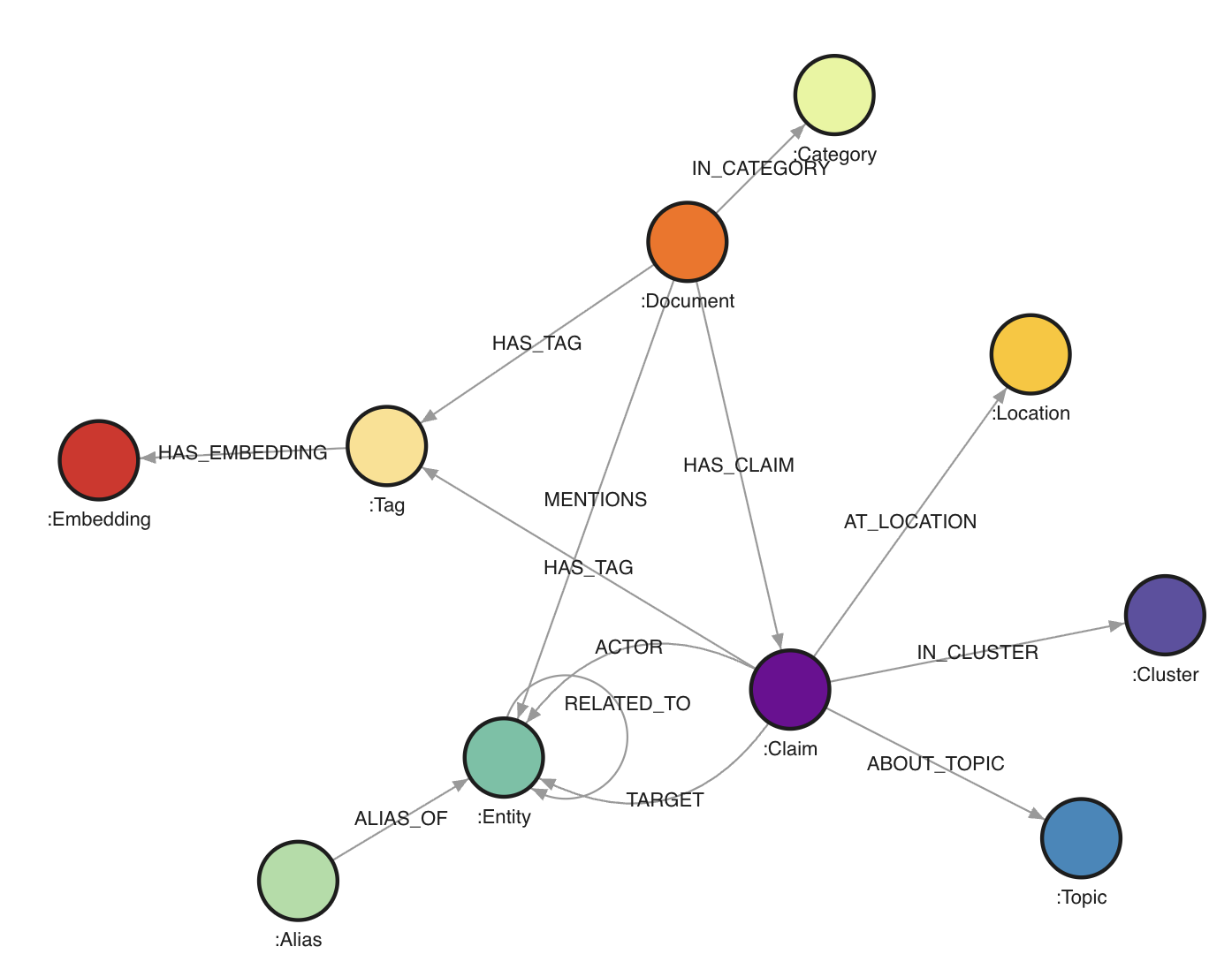The graph contains `546,648` nodes and `1,432,277` edges. Node labels: - `Document` (`25,233`): one source document from the House Oversight dump. Important properties include `doc_id`, `file_path`, `category`, summaries, date range, and the full extracted text. The full text is not necessasy for the core assignment. - `Claim` (`106,012`): one extracted statement or assertion. A claim roughly corresponds to one subject-predicate-object style extraction, with properties such as `claim_id`, `action`, `timestamp`, `sequence_order`, `triple_tags`, `explicit_topic`, `implicit_topic`, and `top_cluster_ids`. - `Entity` (`55,922`): canonical real-world entities such as people, organizations, places, companies, aircraft, properties, and sometimes unresolved named things. - `Alias` (`28,934`): alternative names mapped onto canonical entities. - `Tag` (`109,593`): semantic tags attached either to documents or claims. - `Topic` (`184,695`): explicit or implicit topics inferred for claims. - `Category` (`34`): document categories such as `email`, `report`, `book_excerpt`, `court_filing`, and `photo_caption`. - `Location` (`6,506`): raw location strings linked to claims. - `Cluster` (`30`): coarse topical clusters assigned to claims. - `Embedding` (`29,689`): embeddings linked to tags. These are mostly useful if you want to explore similarity-based extensions, but not necessary for the core assignment. Edge types: - `(:Document)-[:IN_CATEGORY]-﹥(:Category)`: assigns a document to a category. - `(:Document)-[:HAS_TAG]-﹥(:Tag)`: content tags for a document. - `(:Document)-[:HAS_CLAIM]-﹥(:Claim)`: provenance link from a document to extracted claims. - `(:Document)-[:MENTIONS]-﹥(:Entity)`: entity mention relation at document level. - `(:Alias)-[:ALIAS_OF]-﹥(:Entity)`: alias resolution. - `(:Claim)-[:ACTOR]-﹥(:Entity)`: subject/actor side of the extracted relation. - `(:Claim)-[:TARGET]-﹥(:Entity)`: object/target side of the extracted relation. - `(:Claim)-[:AT_LOCATION]-﹥(:Location)`: location attached to a claim. - `(:Claim)-[:HAS_TAG]-﹥(:Tag)`: semantic tags attached to a claim. - `(:Claim)-[:ABOUT_TOPIC {kind: "explicit"|"implicit"}]-﹥(:Topic)`: topics attached to a claim. - `(:Claim)-[:IN_CLUSTER]-﹥(:Cluster)`: cluster membership for a claim. - `(:Entity)-[:RELATED_TO]-﹥(:Entity)`: derived traversal edge between actor and target. This edge contains properties such as `action`, `doc_id`, `claim_id`, `timestamp`, and `sequence_order`. The practical consequence is that you can work at two levels: - the document/evidence level via `Document` and `Claim` - the network level via `Entity` and `RELATED_TO` **Objective** Your task for this assignment is to use Cypher queries and Gephi (or other visualization libraries) to analyze this data set. You are free to explore anything you deem interesting and present your findings in your report. The main goal is to get familiar with Cypher but also to hone your "storytelling" skills. Hence, try to focus on a single or a few hypotheses or findings you explore in full (with nicely formatted visualizations) and explaining what it says instead of just going for quick filter saying: "here are the three nodes with the most connections" (boring) or showing a [graph hairball](https://cambridge-intelligence.com/how-to-fix-hairballs/). Below are some suggestions/tips of what you can go for: - Perform community mining on (a subset of) the graph and see whether you can identify particular groups - Explore the connections between known actors in Epstein's network - Compare document categories: do `court_filing` documents produce a different network structure than `photo_caption` or `email` documents? - Look at recent news stories and see if you can back them or expand on these based on the data set - Compare “social” relations (`attended`, `met`, `traveled with`) with “legal” relations (`testified`, `accused`, `investigated`, `represented`) and see whether the same actors bridge both worlds - Explore centrality, brokerage, or bridge nodes rather than only raw degree - Focus on a single substory, for example aviation, Palm Beach, Mar-a-Lago, financial disclosures, or recruitment pathways I.e. pick something you want to explore and try to work this out in full. You will note that the data set is likely too large to look at everything at once, so a guided “deep dive” will work better. Once you know what you want to focus on, you can also clean up the graph by e.g. removing nodes or edges you are not interested in, or exporting a subgraph (see below). **Setting up Memgraph and Gephi** We used to work with Neo4j for this assignment, which is a solid tool supporting lots of (data science) extensions, but has become so commercial lately that it is a hassle to download. It can also be quite slow. Instead, we’ll be working with Memgraph, which is also “open source but commercial”, but with the advantage that it is faster and easier to set up than Neo4j. It is mostly compatible (e.g. Cypher works the same), but some aspects (such as exporting data) are a bit trickier. Memgraph provides an installer script which sets up a bunch of Docker containers using Docker Compose. Since this is becoming an increasingly common pattern, we can take this opportunity to get (a little bit) familiarized with Docker. First, download and install [Docker Desktop](https://www.docker.com/products/docker-desktop/) for your platform. Pick the free plan and log in with your Google or GitHub account. (Note: also Docker is obviously becoming more and more commercial. There are alternatives available such as [Podman](https://podman.io/) and [Rancher](https://rancherdesktop.io/), but these are a bit harder to set up correctly. Feel free to experiment with these if you want to but you are "on your own" in that case.) Start Docker Desktop once it is installed. If running, you will see an icon in your task bar. Windows users: head to the settings window of Docker Desktop and select the WSL2 backend as the “engine” if possible. It is also a good idea to look under the "Resources" tab and increase the RAM (memory) docker containers can utilize, if you have the memory to spare. You should be able to run the docker command on a command line / Terminal window: ``` docker Usage: docker [OPTIONS] COMMAND A self-sufficient runtime for containers Commands: [A long list of commands] ``` Next, we will NOT use the provided installation script of Memgraph itself but instead use this [docker-compose.yml](./assignment4/docker-compose.yml) file. Download this file and place it in an empty directory of your choosing. You can take a look at this file in a text editor to inspect the configuration it provides. It downloads two images, sets up two containers, exposes the necessary ports, attaches a volume, and sets a `MEMGRAPH` environment variable to increase the query time limit. If necessary, you can increase this limit. In your command line window, navigate (`cd`) to the location where you've placed this file, and run the following command: ``` docker compose up ``` This will take a while the first time. Eventually, you should see the following message: ``` memgraph-lab | [20XX-XX-XX XX:XX:XX] INFO: Lab vX.X.X is running at http://localhost:3000 in production mode ``` Keep this window open to keep Memgraph running. In a web browser, navigate to: [http://localhost:3000/](http://localhost:3000/). The Memgraph lab page should appear and should allow to connect to your locally running Memgraph instance. You can press CTRL+C in the command line window and run `docker compose up` again later to start Memgraph up again, or use the Docker Desktop app to start the two containers from there. You won’t have any nodes or edges (yet). Download the [data.cypherl](https://e.pcloud.link/publink/show?code=XZyqTiZFVoTYYrA6VJGCWIpz1pUQQzrmBtV) data file. Since this file is large, importing it through the web interface will most likely make it crash, so we will use the `mgconsole` program instead. Open a new command line window (whilst Memgraph is still running) and navigate to the directory you downloaded the `data.cypherl` file to. Then run: ``` cat data.cypherl | docker run -i --rm memgraph/mgconsole:latest --host host.docker.internal --port 7687 ``` On Windows, use `type` instead of `cat`. If you are using PowerShell on Windows, the equivalent is: ```powershell Get-Content .\data.cypherl | docker run -i --rm memgraph/mgconsole:latest --host host.docker.internal --port 7687 ``` This should start importing the data. You can verify this by looking at the Memgraph Lab tab in your web browser and seeing the number of nodes and edges increase. The total number of nodes and edges should reach `546,648` and `1,432,277` respectively. This might take some time to finish, but afterwards your data is ready in Memgraph. In case of issues, you can always remove all containers, images and volumes using the Docker Desktop application and run `docker compose up` again. Or you can empty the database using this query: ``` MATCH (n) DETACH DELETE n; ``` Next, [download and install Gephi](https://gephi.org/desktop/) for your OS. **Working with the Graph** You can execute queries in the “Query Execution” pane. Feel free to play around with some Cypher queries to explore this graph, e.g.: ```cypher MATCH (e:Entity)-[r:RELATED_TO]->(f:Entity) RETURN e, r, f LIMIT 25; ``` - It’s a good idea to use limit in order not to overflow yourself with results - Also note that we labeled the edge (`r`) here, otherwise, it will not be shown in the result (this is different from the default behavior from Neo4j which connects nodes) - You can click nodes in the result view to see more info and expand them Some more examples: ```cypher MATCH (d:Document)-[:IN_CATEGORY]->(c:Category) RETURN c.name, count(d) AS n ORDER BY n DESC; ``` ```cypher MATCH (e:Entity {name: "Jeffrey Epstein"})-[r:RELATED_TO]->(other:Entity) RETURN other.name, r.action, r.doc_id LIMIT 50; ``` ```cypher MATCH (d:Document)-[:HAS_CLAIM]->(c:Claim)-[:AT_LOCATION]->(l:Location) WHERE l.name CONTAINS "Palm Beach" RETURN d.doc_id, c.action, l.name LIMIT 50; ``` ```cypher MATCH (c:Claim)-[:ABOUT_TOPIC {kind: "explicit"}]->(t:Topic) RETURN t.name, count(*) AS n ORDER BY n DESC LIMIT 25; ``` ```cypher MATCH (a:Alias)-[:ALIAS_OF]->(e:Entity) RETURN e.name, count(a) AS alias_count ORDER BY alias_count DESC LIMIT 25; ``` ```cypher MATCH (d:Document)-[:HAS_CLAIM]->(c:Claim)-[:ACTOR]->(a:Entity) MATCH (c)-[:TARGET]->(b:Entity) RETURN d.doc_id, a.name, c.action, b.name LIMIT 25; ``` Notice that the graph supports different styles of querying: - `Document` and `Claim` for provenance and evidence - `Entity` and `RELATED_TO` for social-network style analysis - `Tag`, `Topic`, and `Category` for semantic filtering You can change size and color of the node types as well as the attribute used to label them by going to the “Graph Style Editor” tab. Memgraph’s styling language is quite powerful. For more information, check out: [https://memgraph.com/blog/how-to-style-your-graphs-in-memgraph-lab](https://memgraph.com/blog/how-to-style-your-graphs-in-memgraph-lab). **Using Gephi** To load the data in Gephi, we must get it out of Memgraph in some manner. There is a Neo4j Gephi plugin, but it has not received much attention lately and is incompatible with Memgraph. Luckily, there is an export function to JSON from a query result from the web interface. To export query results from Memgraph Lab: run a query or select results you want to export. Click Export results and choose JSON. This file can then be converted using the [json2graphml.py](./assignment4/json2graphml.py) Python script (note that you will need the networkx package): ``` uv run --with networkx json2graphml.py "memgraph-query-results-export.json" Done, output file saved to: memgraph-query-results-export.graphml ``` (Note that this script attempts to perform a best-effort conversion and might not be 100% foolproof depending on the query you used.) Feel free to use other Python (or JavaScript) libraries to make visualizations as well if you prefer these over Gephi. Memgraph itself has a good article with some tips over at [https://memgraph.com/blog/graph-visualization-in-python](https://memgraph.com/blog/graph-visualization-in-python). **Exporting CSV Files** To load data into Gephi, another workflow consists of creating: - one CSV file with nodes - one CSV file with edges For example, you might first export the edges of a focused subgraph: ```cypher WITH " MATCH (a:Entity)-[r:RELATED_TO]->(b:Entity) WHERE a.name CONTAINS 'Epstein' OR b.name CONTAINS 'Epstein' RETURN a.name AS source, b.name AS target, r.action AS action, r.doc_id AS doc_id LIMIT 1000 " AS query CALL export_util.csv_query(query, "/var/lib/memgraph/edges.csv", True) YIELD file_path RETURN file_path; ``` Then export the corresponding nodes: ```cypher WITH " MATCH (e:Entity) WHERE e.name CONTAINS 'Epstein' RETURN e.name AS id, e.name AS label, e.entity_type AS entity_type LIMIT 500 " AS query CALL export_util.csv_query(query, "/var/lib/memgraph/nodes.csv", True) YIELD file_path RETURN file_path; ``` After copying the files out of the container (see below), you can import them into Gephi via the Data Laboratory: - import `nodes.csv` as a nodes table - import `edges.csv` as an edges table - make sure the source/target columns refer to the node ids you exported It is recommended to run these commands in a terminal window rather than from the web interface. How do you get a terminal query prompt to Memgraph? By executing the following command in a separate Terminal window: On Linux: ``` docker run -it --rm --network host memgraph/mgconsole:latest ``` On macOS or Windows: ```bash docker run -it --rm memgraph/mgconsole:latest --host host.docker.internal --port 7687 ``` (Note the `-it` instead of just `-i` earlier). A prompt will open on which you can execute queries: ``` memgraph: WITH "[YOUR QUERY HERE]" AS query CALL export_util.csv_query(query, "/var/lib/memgraph/my_export.csv", True) YIELD file_path RETURN file_path; +-------------------------------------------------+ | file_path | +-------------------------------------------------+ | "/var/lib/memgraph/my_export.csv" | +-------------------------------------------------+ 1 row in set (round trip in 0.118 sec) ``` We use `/var/lib/memgraph/` as the path to export to. Note that this location is inside of the docker container. So how to get it out? We can copy the file as follows: ``` docker cp bd6b5372d713:/var/lib/memgraph/my_export.csv my_export.csv Successfully copied 24.6kB to G:\my_export.csv ``` You will have to replace the identifier `bd6b5372d713` with the one on your machine. You can get this identifier by running `docker ps` and getting the id for `memgraph/memgraph-mage:latest`. The file is then present on your local environment. In practice, exporting focused node and edge CSV files is usually the easiest route into Gephi. In practice, for this assignment, the best approach is usually: 1. formulate a small, targeted Cypher query 2. export only the resulting subgraph 3. visualize and refine That approach is much better than dumping the entire graph into Gephi and ending up with an unreadable hairball. *You do not hand in each assignment separately, but hand in your completed lab report containing all four assignments on Sunday May 31st. For an overview of the groups, see Toledo. Note for externals (i.e. anyone who will NOT partake in the exams -- this doesn't apply to normal students): you are free to partake in (any of) the assignments individually, but not required to.* # Course 12: May 11 ## Slides * Continuing with the slides of last time ## Recording * [YouTube](https://youtu.be/9byvcPsKHzk) ## Background Information [In the news](./news/News_05-11.pptx) (slides) Extra references: * [Network visualization of 50k blogs and links](https://news.ycombinator.com/item?id=40136208) * [I Made a Graph of Wikipedia... This Is What I Found](https://www.youtube.com/watch?v=JheGL6uSF-4) * [Y'all Are Nerds (According to Math)](https://www.youtube.com/watch?v=o879xRxmwmU&t=216s) * PageRank, personalized PageRank, and others: [1](https://www.r-bloggers.com/from-random-walks-to-personalized-pagerank/), [2](http://www.cs.princeton.edu/~chazelle/courses/BIB/pagerank.htm), [3](http://www.math.ucsd.edu/~fan/wp/lov.pdf), [4](http://www.cs.yale.edu/homes/spielman/462/2010/lect16-10.pdf) * The [docs of igraph](http://igraph.org/r/doc/) contain a good overview of available centrality, betweenness, ... metrics and community mining * Node2vec: [http://snap.stanford.edu/node2vec/](http://snap.stanford.edu/node2vec/) * GraphSAGE: [https://github.com/williamleif/GraphSAGE](https://github.com/williamleif/GraphSAGE) * Deepwalk: [https://arxiv.org/abs/1403.6652](https://arxiv.org/abs/1403.6652) * [Journal paper discussing the popular ForceAtlas2 technique](http://journals.plos.org/plosone/article?id=10.1371/journal.pone.0098679) * [Another paper detailing simple and less simple layout techniques](http://profs.etsmtl.ca/mmcguffin/research/2012-mcguffin-simpleNetVis/mcguffin-2012-simpleNetVis.pdf) * [Examples to play with in the browser](https://bl.ocks.org/steveharoz/8c3e2524079a8c440df60c1ab72b5d03) * [GraphViz](http://www.graphviz.org/) is a standalone tool for graph-based visualizations and layout, which are described by means of the DOT language. It has lots of bindings with programming languages available and is still widely used as a behind-the-scenes layout driver in many products * igraph is a graph analysis package for R and Python: [http://igraph.org/](http://igraph.org/) * Others: [http://js.cytoscape.org/](http://js.cytoscape.org/), [http://sigmajs.org/](http://sigmajs.org/) and [http://visjs.org/](http://visjs.org/) * [NetworkX](https://networkx.github.io/) is a Python package for graph analysis * Spark's [GraphX](http://spark.apache.org/graphx/) and [GraphFrames](https://graphframes.github.io/) * [Gephi](https://gephi.org/) is a tool for graph layout, analysis and visualisation * Also see the [ggraph](https://cran.r-project.org/web/packages/ggraph/index.html), [ggnet2](https://briatte.github.io/ggnet/), [sna](https://cran.r-project.org/web/packages/sna/index.html), [network](https://cran.r-project.org/web/packages/network/index.html), [tidygraph](https://github.com/thomasp85/tidygraph) packages in R * [Pytorch Geometric](https://pytorch-geometric.readthedocs.io/en/latest/) * Neo4j: [https://neo4j.com/](https://neo4j.com/) * Memgraph: [https://memgraph.com/](https://memgraph.com/) * OrientDB: [http://orientdb.com/orientdb/](http://orientdb.com/orientdb/) * SparkSee: [http://www.sparsity-technologies.com/](http://www.sparsity-technologies.com/) * FlockDB: [https://github.com/twitter-archive/flockdb](https://github.com/twitter-archive/flockdb) * Titan: [http://titan.thinkaurelius.com/](http://titan.thinkaurelius.com/) * AllegroGraph: [https://franz.com/agraph/allegrograph/](https://franz.com/agraph/allegrograph/) * InfiniteGraph: [http://www.objectivity.com/products/infinitegraph/](http://www.objectivity.com/products/infinitegraph/) * EdgeDB: [https://www.edgedb.com/](https://www.edgedb.com/) * TinkerPop and Gremlin: [https://tinkerpop.apache.org/gremlin.html](https://tinkerpop.apache.org/gremlin.html) * Intro to Cypher: [https://memgraph.com/docs/cypher-manual/](https://memgraph.com/docs/cypher-manual/) and [https://neo4j.com/developer/cypher-query-language/](https://neo4j.com/developer/cypher-query-language/) * [Efficient graph algorithms on Neo4j](https://neo4j.com/blog/efficient-graph-algorithms-neo4j/): build-in solution * [Data science library on Neo4j](https://neo4j.com/graph-data-science-library/): build-in, newer solution * [MAGE - Memgraph Advanced Graph Extensions](https://memgraph.com/docs/mage) * Neo4j use cases: [https://neo4j.com/graphgists/](https://neo4j.com/graphgists/) and [https://neo4j.com/sandbox/](https://neo4j.com/sandbox/) # Resources ## Books If you want an exhaustive list of data science books (not required for the course), feel free to check out: - [https://github.com/MasoudKaviani/freemachinelearninigbooks](https://github.com/MasoudKaviani/freemachinelearninigbooks) - [https://github.com/chaconnewu/free-data-science-books](https://github.com/chaconnewu/free-data-science-books) - [https://github.com/bradleyboehmke/data-science-learning-resources](https://github.com/bradleyboehmke/data-science-learning-resources) - [https://github.com/Saurav6789/Books-](https://github.com/Saurav6789/Books-) - [https://github.com/yashnarkhede/Data-Scientist-Books](https://github.com/yashnarkhede/Data-Scientist-Books) ## Python Tutorials Python itself is [quite easy](https://learnxinyminutes.com/docs/python/); you mainly need to figure out the additional libraries and their usage. Try to become familiar with `Numpy`, `Pandas`, and `scikit-learn` first, e.g. [play along with a couple of these examples](https://scikit-learn.org/stable/auto_examples/index.html). The bottom of [this page](https://learnxinyminutes.com/docs/python/) also lists some more resources to learn Python. The following are quite good: * [A Crash Course in Python for Scientists](https://nbviewer.jupyter.org/gist/anonymous/5924718) * [Dive Into Python 3](https://diveintopython3.net/index.html) * [https://docs.python-guide.org/](https://docs.python-guide.org/) (a bit more intermediate) * Someone has also posted [this 100 Page Python Intro](https://learnbyexample.github.io/100_page_python_intro/introduction.html) ## DataCamp To get access to DataCamp, use this [registration link](https://www.datacamp.com/groups/shared_links/67256766fea5a442a7217822450f1fd5d83a7f46711f8a90f06348f5c1de0d61). You can use this classroom to get access to courses to enhance your learning. Note that this will require a @(student.)kuleuven.be email address. If you'd like to use a personal email instead (e.g. because you already have an account on DataCamp), send me an email.